Scooby-Doo Analytics Presents
Ruh-Roh Raggy: Look out for that Random Forest!
Introduction
“Scooby-Doo, Where Are You!” first aired on television screens in 1969, captivating viewers with a unique blend of mystery, humor, and lovable characters. This iconic series not only enjoyed a successful run until 1986 but also inspired spin-offs and movies, including a “A Pup Named Scooby-Doo” from 1988 to 1991. Chances are, you, the reader, hold fond memories of watching Scooby-Doo, whether it be Saturday morning chartoons during your childhood or now, alongside your children.
Thankfully, the world of Scooby-Doo offers more to us than just nostalgia; we have a rich dataset begging to be analyzed for a grad-student’s homework assignment. Thanks to plummye for spending an entire year performing manual data gathering, we have an amazing 603 record, 75 feature dataset. This dataset includes information on episode run-times, the broadcasting network, monster types, popular catchphrases and the number of Scooby Snacks consumed.
Dear reader, my point is we have an amazing dataset full of nostalgia and the plan is to take a trip down memory lane with an analytical spin.
WARNING: There will be an over-use of puns that you will not understand if you’ve never watched Scooby-Doo. For those of you interested, you can find the original series episodes here.
It looks like we’ve got ourselves a mystery.
Our task today? None other than to predict the unpredictable, to forecast the unseen, much like trying to guess the monster lurking in the shadows. Our adventure has led us to predicting the imdb score for each of our Scooby-Doo episodes.
Like any good detective gang, we have a few methods for apprehending the best approach. Below is a list of our potential models as well as some of the hyperparameters that we will tune:
- Linear Regression - No tuning needed
- Elastic net
- Penalty - magnitude of regularization
- Mixture - balance between lasso/ridge
- KNN
- Number of Neighbors
- SVM
- Cost - controlls the error term penalty
- Kernel - type of function to be used to transform into higher dimensional space
- Random Forest
- # of Trees - Number of trees to be used
- mtry - Number of variables considered for splitting at each leaf node
- min_n - Minimum number of samples required to split an internal node
- Boosted (XGBoost)
- # of Trees - Number of trees to be used
- Tree Depth - Maximum depth of the trees
- min_n - Minimum number of samples required to split an internal node
- Learning Rate - adjusts conservative nature of the boosting process
Adjusting each of these hyperparameters and choosing the best model should be the best approach to creating an accurate and reliable model that predicts the IMDb score for each episode.
The “I fast-forwarded to the end of the episode” Summary
Sometimes you are watching a show and are just clamoring for what’s at the end. Luckily for you, I’m giving you an Executive Summary here.
- This is a very high dimensional yet small in size dataset (potential for 250+ predictors with only 600 movie records)
- Overfitting is highly likely due to the dimensionality
- Feature selection could be improved upon in future analysis to combat some of the overfitting
- Principal component analysis could be utilized
- Overfitting is highly likely due to the dimensionality
- Some computations take a long time to run (10+ minutes) even with parallel processing
- Leads to issues if used on a production server
- Monetary and Environmental cost considerations
- Random Forest performs best across the board!
- XGBoost performs in-line with other baseline models but not as good as Random Forest
- Slow run-times due to the number amount of hyper-parameter tuning
- Performance lacks due to the very minimal amount of training data (470 observations for training; 118 for testing)
- Ensemble method performs near Random Forest levels and should provide a robust and reliable model for future IMDb predictions
- Should help with overfitting concerns
With this high level summary, let’s dive into some exploration of the data
My glasses! I can’t see the data without my glasses!
Gotta love Velma’s iconic line! She tends to lose her glasses in episodes and is always searching for them! It would certainly be pretty hard for her to see and understand the data without them!
Let’s first get an understanding of the breadth of our Scooby-Doo data. There are a plethora of predictors in this dataset ranging from the types of monsters to the catchphrases used and the number of scooby snacks eaten. Let’s take a look at some in the visuals and discuss how they might be useful to a model for the IMDb score.
Initial Dimensionality
As stated before, the dataset has many potential dimensions. Below in Table 1 we see that there are 603 records and 75 features. This is a very small dataset for analysis but, at least it is fun and we are recognizing the downsides…
The number of predictors balloons to well over 200 when performing one-hot encoding and additional feature engineering-methods.
Episodes Per Series
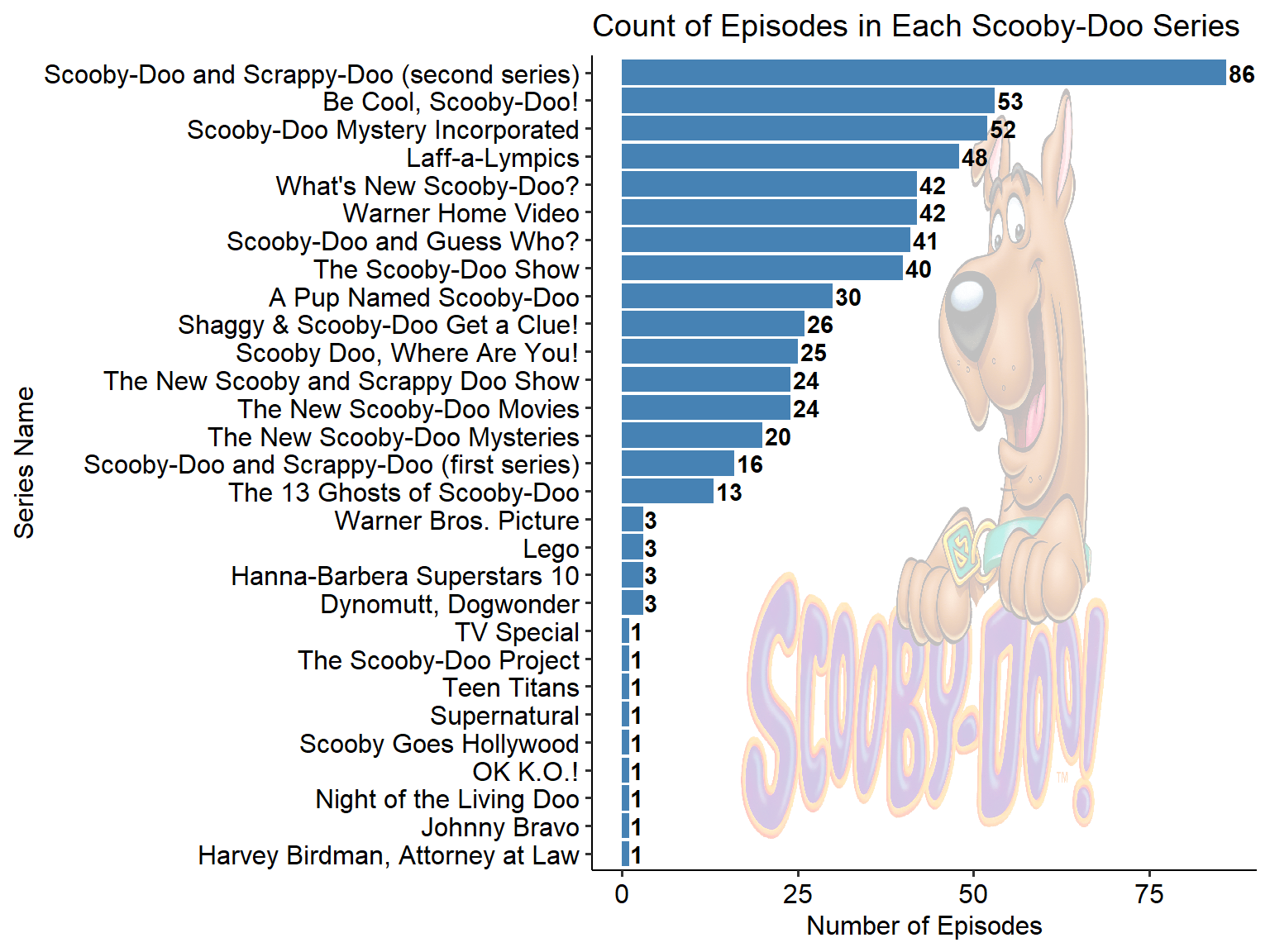
Graphically, let’s start off with the episodes per series. We want to look at this to know specifically if there could be a bias towards a particular series.
Figure 1 shows us that Scooby-Doo and Scrappy-Doo (The second series) has the most episode listed in our dataset. There are also a lot of one-off special episodes such as a lego crossover and a Supernatural crossover! Jinkies!
My suggestion would be to remove any of these series with less than 10 observations in total. With this field being more categorical, it would be a lot more difficult for a model to pick up on the subtleties of the data for these very low observation types of series. However, if removing the data is not desired, you can also group these series into an “Other” category and proceed with the analysis or use a flag for “crossover” which is conveniently in our dataset.
Popular Phrases
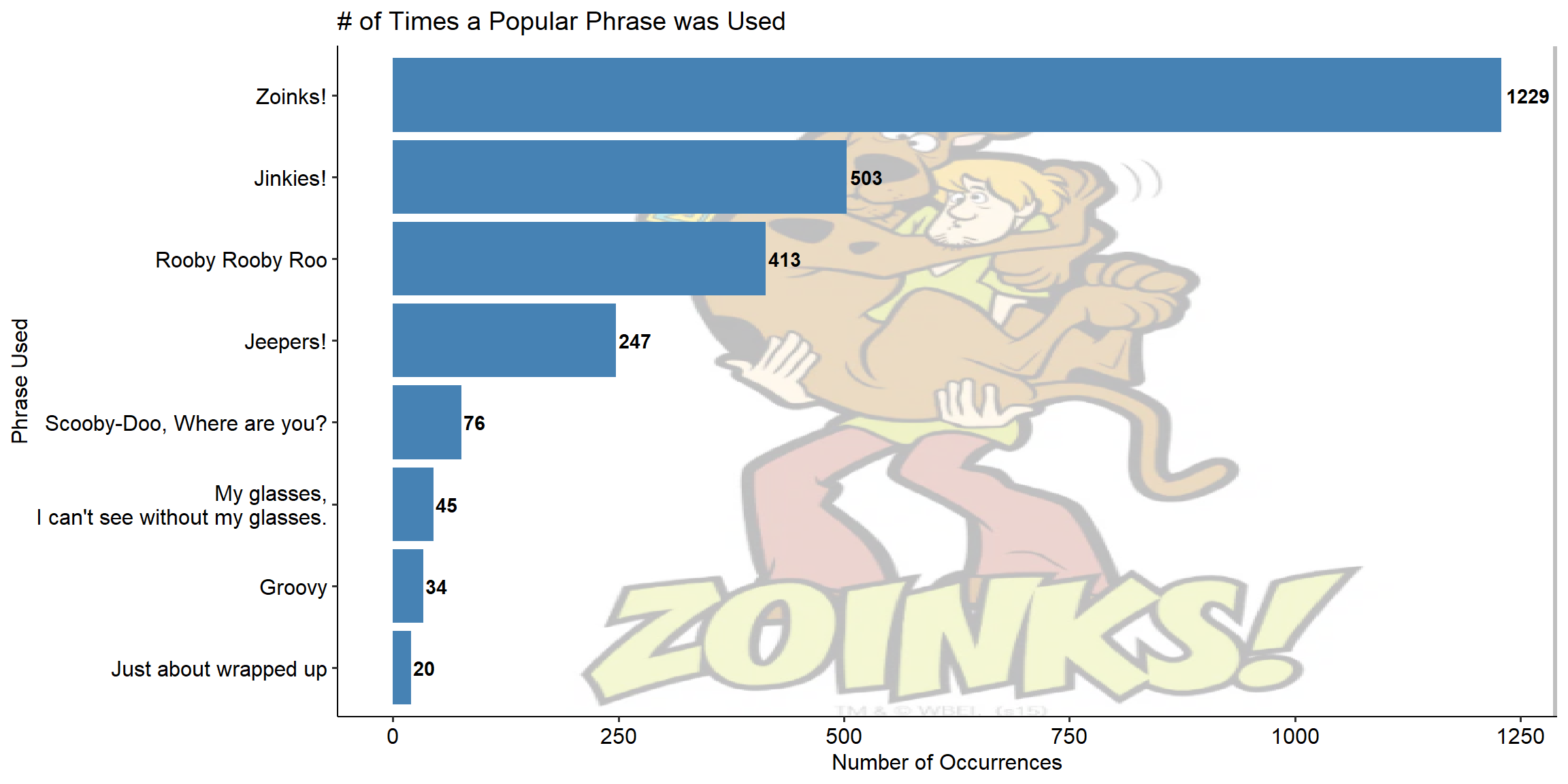
Scooby-Doo wouldn’t be as iconic without its popular phrases. From Zoinks! to Jeepers! or My Glasses!, each episode is filled with at least a handful of the overall series popular catchphrases.
These phrases appear during times of stress (Rikes), to times of discovery (Jinkies) to signaling the end of the mystery (Just about wrapped up). Each is as unique as the character that says it.
Figure 2 gives us an idea of how often those phrases were used in our dataset. Zoinks is by far the most popular and was typically used by Shaggy when he was scared or surprised. My guess is that due to the fact that it is used in a majority of episodes will lead it to have less predictive power over in terms of a categorical Is Used or Isn’t Used. Others like Groovy seem to be more tactically used and could signify an episode’s significance.
Unmasking the Bad Guy
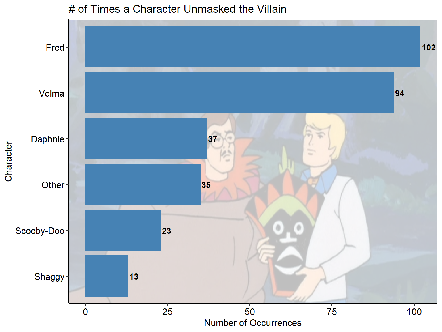
Like any good detective show, it always feels good to be able to unmask the bad guy. Figure 3 shows us who typically gets to do the unmasking, Fred and Velma are by far the runaways here unmasking in almost a third of the shows between the two.
Regardless of who does the unmasking, the build up to the unmasking is generally the most exciting but nevertheless, unmasking may be important to the IMDb score.
Potential Additional Exploration
This Scooby-Doo dataset has a well over 100 potential parameters after feature engineering. It would be impossible to investigate each for the purposes of this assignment. I will include some additional ideas for exploration within the Next Steps section (Next time on Scooby-Doo Analytics).
Jinkies, I’ve found the models!
How we got here
As shown before, the plan was to create models for Linear Regression, KNN, SVM, Random Forest and Boosted trees via XGBoost. For this analysis I used the tidymodels framework. Please see the attached code for a reference on that framework. The cross-validation and hyperparameter tuning is baked entirely into the tidymodels framework to make for a relatively easy process.
I chose to do 5-fold cross validation in addition to an 80/20 train/test split. This dataset is a relatively small dataset overall with only 600 or so initial episode records. Once we remove missing values we are closer to the 550 mark. Our training set is very small compared to what would typically be advised. We are very likely to overfit regardless of the cross-validation and parameter tuning that is done. Nevertheless, we will throw the kitchen sink at it anyways!
Cross-validation Example
As mentioned before, we performed 5-fold cross-validation as well as grid search hyperparameter tuning. Table 2 displays the grid-search parameters and the associated metric estimates. I’ve set the final model to be chosen based upon minimizing the rmse. Other metrics could be chosen as desired. This process is repeated 4 times and then the best .config is chosen containing the tuned hyperparameters.
| mtry | trees | min_n | .metric | .estimator | .estimate | .config |
|---|---|---|---|---|---|---|
| 4 | 983 | 7 | rmse | standard | 0.5620380 | Preprocessor1_Model001 |
| 4 | 983 | 7 | rsq | standard | 0.6655370 | Preprocessor1_Model001 |
| 6 | 546 | 3 | rmse | standard | 0.5023651 | Preprocessor1_Model002 |
| 6 | 546 | 3 | rsq | standard | 0.7066864 | Preprocessor1_Model002 |
| 11 | 644 | 10 | rmse | standard | 0.4575371 | Preprocessor1_Model003 |
| 11 | 644 | 10 | rsq | standard | 0.7353098 | Preprocessor1_Model003 |
| 5 | 849 | 5 | rmse | standard | 0.5288565 | Preprocessor1_Model004 |
| 5 | 849 | 5 | rsq | standard | 0.6894134 | Preprocessor1_Model004 |
| 14 | 351 | 8 | rmse | standard | 0.4323569 | Preprocessor1_Model005 |
| 14 | 351 | 8 | rsq | standard | 0.7625322 | Preprocessor1_Model005 |
Model Results
Our final model results are displayed in Table 3 and overall we have found that the Random Forest Regression performs the best in terms of RMSE and MAE. However, perhaps a more robust approach would be to use the ensemble method as it performs very well but is a combination of all models listed, reducing the chances of overfitting our dataset.
From what we see in this table, the boosted tree models performed very poorly. My initial reaction to this was surprised but upon additional research I found that the XGBoost model tends to overfit when faced with a very small dataset with lots of predictors. This is certainly the case, especially considering our large number of 2-3 label factor variables being used.
All models perform better than a baseline linear regression model and overall it seems as if the Random Forest model was well-worth training as we see nearly a 10% or more decrease in MAE compared to most other models.
| Model | RunTime | rmse | rsq | mae |
|---|---|---|---|---|
| Random Forest Regression | 86.814793 | 0.4945017 | 0.5484139 | 0.3202019 |
| Ensemble Average | NA | 0.5035838 | 0.5263849 | 0.3245341 |
| SVM Regression | 14.165173 | 0.5036852 | 0.5299300 | 0.3415585 |
| Elastic Net Regression | 59.881784 | 0.5427669 | 0.5035292 | 0.3701625 |
| KNN Regression | 6.084439 | 0.5574041 | 0.4240404 | 0.3775733 |
| Boosted w/ Regular Grid Search | 617.337236 | 0.5878516 | 0.4222285 | 0.3789965 |
| Boosted w/ Hypercube Grid Search | 683.588239 | 0.6089094 | 0.3813681 | 0.3975507 |
| Linear Regression | 1.276290 | 0.8247458 | 0.2905084 | 0.5052055 |
Model Run-time
I wanted to include this section because it is very noteworthy that Table 3 has the run-time for each model displayed. In the case of our boosted models, they took roughly 10+ minutes to run for very minimal gains. The Random Forest was roughly a minute and a half run-time on average and ended up being the best model. This run-time is effected by the number of parameters being tuned as well as the overall amount of cross-validation. While in this instance, XGBoost was slow and showed minimal performance gains, it does not always mean this will be the case. Nevertheless, it is important to consider factors such as the run-time of a model. Longer run-times require more compute resources which could in return drive up cost both economically and environmentally. It is important to be cautious of the models running and the parameters being tuned and weigh the benefits of putting something into production that may have a longer run-time. For our project here, I would likely not pursue the boosted model in production without attempting to reduce the run-time.
This Mystery is Starting to come Together!
Scooby-Dooby-Doo!
It wouldn’t be a Scooby-Doo themed paper without wrapping it up with the iconic “Scooby-Dooby-Doo” quote! Typically Scoobs would shout this towards the end of an episode as a joyous celebration.
I think we can joyously shout “Scooby-Dooby-Doo”! With this analysis we’ve examined a few potentially key features for analysis. We tested numerous models (Linear regression, KNN, SVM, and tree-based models) used both cross-validation and grid-search for hyperparameter tuning and finally found our best performing model to be the random forest model. The results were a little surprising, particularly that the boosted models performed as poorly as they did and with extreme run-times but that is likely due to the large number of parameters being tuned and the relatively small dataset used.
Next time on Scooby Doo Analytics
Future analysis could expand upon the feature engineering done for this analysis. Most predictors were treated as factor variables due to the nature of the dataset.
Additional manual entry could be performed to fill in the gaps for the numerous NULL values across predictors.
More tuning of the boosted models could be done to find the right parameters that improve the errors and run-times to more appropriate levels.


